Texture Mapping
This is an online bonus chapter for The Ray Tracer Challenge, by Jamis Buck. To be successful, you:
should have an account at the Ray Tracer Challenge forum. Ask all your questions there, and see how others have managed!
must have a copy of The Ray Tracer Challenge.
must have implemented your ray tracer through chapter 10 ("Patterns").
If you don't have a copy of the book, grab one today and start writing a 3D renderer of your own!
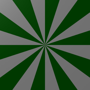
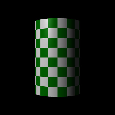
By now, you've probably tried applying a 3D solid checker pattern (like what you implemented in chapter 10, "Patterns") to a sphere. The result—as mentioned in the book—is disappointing, as if you'd carved the sphere from a checkered block of stone.
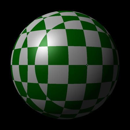
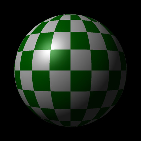
It really doesn't look very nice. To correctly apply a pattern to the surface of a sphere (or any curved surface), you need to essentially unwrap the surface so it lies flat, in two dimensions, and then apply the pattern to that two-dimensional surface. If you do, the result is a bit more pleasing:
This is exactly what you'll learn how to do in this chapter. First, you'll implement a two-dimensional checker pattern and map it onto a sphere. Then, generalizing your technique a bit, you'll map that same pattern onto a plane, and then a cylinder, and then move on to cube mapping. You'll wrap things up with an implementation of a simplified PPM parser (kind of the opposite of what you built in chapter 2, "Drawing on a Canvas"), and use it to map actual images onto your shapes, unlocking all kinds of possibilities for your scenes.
Let's get to it!
2D Checkers on a 3D Sphere
Two-dimensional patterns and three-dimensional patterns have a lot in common. Fundamentally, they are functions that accept a position as input, and return a color. With the three-dimensional patterns you implemented in the book, the positions you passed to the pattern were three-dimensional. It should come as no surprise, then, that the positions you pass to the two-dimensional patterns are two-dimensional points.
Talking about two- and three-dimensional points in the same breath can get confusing, though. Which x and y are we talking about? For that reason, we'll refer to the components of a two-dimensional point as u and v, and reserve x, y, and z for the three-dimensional points.
For example, here's a 2D checkers pattern, described in terms of u and v:
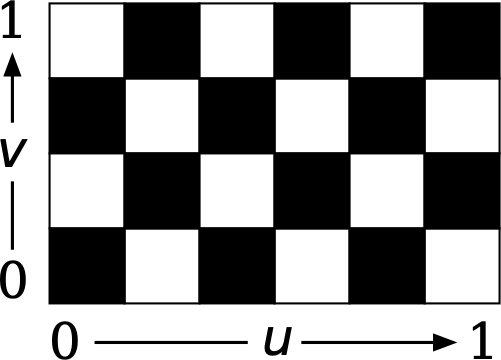
For this and all other 2D patterns in this chapter, you may assume that u and v both have ranges of 0 to 1 (inclusive). At the bottom-left corner of the checkers pattern above, u and v are both 0. At the top-right corner, they are both 1.
In the case of a checkers pattern, you also need to be able to specify how many squares the pattern consists of. The width of the pattern is the number of squares in u, and the height is the number of squares in v. For the previous diagram, the pattern has a width of 6, and a height of 4.
Let's make this real. Add a new function, uv_checkers(width, height, color_a, color_b), which will return a data structure that encapsulates the function's parameters. The width and height parameters describe how many squares the pattern creates in u and v, and color_a and color_b are the colors of the squares. Then another function, uv_pattern_at(pattern, u, v) will return the pattern's color at the given u and v coordinates, where both u and v are floating point numbers between 0 and 1, inclusive.
Here's a test that demonstrates both functions in action.
patterns.featureScenario Outline: Checker pattern in 2D
  Given checkers ← uv_checkers(2, 2, black, white)
  When color ← uv_pattern_at(checkers, <u>, <v>)
  Then color = <expected>

  Examples:
    | u   | v   | expected |
    | 0.0 | 0.0 | black    |
    | 0.5 | 0.0 | white    |
    | 0.0 | 0.5 | white    |
    | 0.5 | 0.5 | black    |
    | 1.0 | 1.0 | black    |
That uv_pattern_at() function will multiply u and v by (respectively) the width and height of the pattern, round each down to the nearest whole number, and add them together. If the result modulo 2 is zero, return color_a. Otherwise, return color_b.
Here's pseudocode:
function uv_pattern_at(checkers, u, v)
  let u2 ← floor(u * checkers.width)
  let v2 ← floor(v * checkers.height)

 if (u2 + v2) mod 2 == 0 then
   return checkers.color_a
 else
   return checkers.color_b
 end if
end function
Once that test is passing, the next step is to tell your renderer how to map a 3D point (x, y, z) on the surface of sphere to a 2D point (u, v) on the flattened surface. You'll introduce a new function, spherical_map(p), which returns the (u, v) pair corresponding to the given 3D point p.
The behavior we want is for u to increase from 0 to 1 as you move counter-clockwise around the sphere, and for v to increase from 0 to 1 as you go from the south pole to the north pole.
Here's a test, making those expectations concrete:
patterns.featureScenario Outline: Using a spherical mapping on a 3D point
  Given p ← <point>
  When (u, v) ← spherical_map(p)
  Then u = <u>
    And v = <v>

  Examples:
    | point                | u    | v    |
    | point(0, 0, -1)      | 0.0  | 0.5  |
    | point(1, 0, 0)       | 0.25 | 0.5  |
    | point(0, 0, 1)       | 0.5  | 0.5  |
    | point(-1, 0, 0)      | 0.75 | 0.5  |
    | point(0, 1, 0)       | 0.5  | 1.0  |
    | point(0, -1, 0)      | 0.5  | 0.0  |
    | point(√2/2, √2/2, 0) | 0.25 | 0.75 |
Here, p is assumed to lie on the surface of a sphere centered at the origin. Whatever distance p is from the origin, that's the radius of the sphere. From here, it's a matter of some trigonometry to convert that 3D point to spherical coordinates, and then convert those spherical coordinates into a (u, v) pair.
That's a mouthful!
Here's some pseudocode for the spherical_map() function.
function spherical_map(p)
  # compute the azimuthal angle
  # -π < theta <= π
  # angle increases clockwise as viewed from above,
  # which is opposite of what we want, but we'll fix it later.
  let theta ← arctan2(p.x, p.z)

  # vec is the vector pointing from the sphere's origin (the world origin)
  # to the point, which will also happen to be exactly equal to the sphere's
  # radius.
  let vec ← vector(p.x, p.y, p.z)
  let radius ← magnitude(vec)

  # compute the polar angle
  # 0 <= phi <= π
  let phi ← arccos(p.y / radius)

  # -0.5 < raw_u <= 0.5
  let raw_u ← theta / (2 * π)

  # 0 <= u < 1
  # here's also where we fix the direction of u. Subtract it from 1,
  # so that it increases counterclockwise as viewed from above.
  let u ← 1 - (raw_u + 0.5)

  # we want v to be 0 at the south pole of the sphere,
  # and 1 at the north pole, so we have to "flip it over"
  # by subtracting it from 1.
  let v ← 1 - phi / π

  return (u, v)
end function
The two-argument arctangent function (possibly called arctan2 or atan2) and the arccosine (arccos or acos) function can probably be found in your language's mathematics module.
Okay, once that test is passing, you're almost ready to render something with this. The next step is to create a Pattern subclass (like your stripes, rings, or gradient patterns) that uses these functions to texture the surface of a sphere. Write a function texture_map(uv_pattern, uv_map), which returns a new TextureMap pattern instance that encapsulates the given uv_pattern (like uv_checkers()) and uv_map (like spherical_map()).
Here's a test, showing how the new pattern works with a smattering of random points on a unit sphere:
patterns.featureScenario Outline: Using a texture map pattern with a spherical map
  Given checkers ← uv_checkers(16, 8, black, white)
    And pattern ← texture_map(checkers, spherical_map)
  Then pattern_at(pattern, <point>) = <color>

  Examples:
    | point                            | color |
    | point(0.4315, 0.4670, 0.7719)    | white |
    | point(-0.9654, 0.2552, -0.0534)  | black |
    | point(0.1039, 0.7090, 0.6975)    | white |
    | point(-0.4986, -0.7856, -0.3663) | black |
    | point(-0.0317, -0.9395, 0.3411)  | black |
    | point(0.4809, -0.7721, 0.4154)   | black |
    | point(0.0285, -0.9612, -0.2745)  | black |
    | point(-0.5734, -0.2162, -0.7903) | white |
    | point(0.7688, -0.1470, 0.6223)   | black |
    | point(-0.7652, 0.2175, 0.6060)   | black |
The pseudocode for the pattern_at(texture_map, point) function comes together like this:
function pattern_at(texture_map, point)
  let (u, v) ← texture_map.uv_map(point)
  return uv_pattern_at(texture_map.uv_pattern, u, v)
end function
And when that test is passing, you'll be able to render your first properly checkered sphere!
checkered-sphere.yml- add: camera
  width: 400
  height: 400
  field-of-view: 0.5
  from: [0, 0, -5]
  to: [0, 0, 0]
  up: [0, 1, 0]

- add: light
  at: [-10, 10, -10]
  intensity: [1, 1, 1]

- add: sphere
  material:
    pattern:
      type: map
      mapping: spherical
      uv_pattern:
        type: checkers
        width: 20
        height: 10
        colors:
          - [0, 0.5, 0]
          - [1, 1, 1]
    ambient: 0.1
    specular: 0.4
    shininess: 10
    diffuse: 0.6
If you want your checkers to look "square" on the sphere, be sure and set the width to twice the height. This is because of how the spherical map is implemented. While both u and v go from 0 to 1, v maps 1 to π, but u maps 1 to 2π.
Fantastic. Let's look at a couple of other mappings next: planar, and cylindrical.
Planar and Cylindrical mappings
That spherical mapping works great...on spheres. It's not so great on other shapes. Check it out:
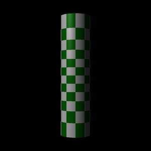
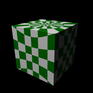
The plane doesn't look anything like a checker pattern. The cylinder...actually doesn't look terrible, but the checker pattern is visibly distorted toward the ends. And the cube, well... Let's just say it's possible to do much, much better.
Let's start by describing a planar mapping.
Planar Mapping
Just as the spherical mapping took 3D points from the surface of a sphere and mapped them onto a 2D surface, the planar mapping will map 3D points from the surface of a plane. However, since a plane is already basically a 2D surface, you may guess (correctly!) that there's not much for such a mapping to do.
Here's a test, which almost gives the whole thing away by itself:
patterns.featureScenario Outline: Using a planar mapping on a 3D point
  Given p ← <point>
  When (u, v) ← planar_map(p)
  Then u = <u>
    And v = <v>

  Examples:
    | point                   | u    | v    |
    | point(0.25, 0, 0.5)     | 0.25 | 0.5  |
    | point(0.25, 0, -0.25)   | 0.25 | 0.75 |
    | point(0.25, 0.5, -0.25) | 0.25 | 0.75 |
    | point(1.25, 0, 0.5)     | 0.25 | 0.5  |
    | point(0.25, 0, -1.75)   | 0.25 | 0.25 |
    | point(1, 0, -1)         | 0.0  | 0.0  |
    | point(0, 0, 0)          | 0.0  | 0.0  |
The idea behind this test is that the planar mapping tiles every unit square on the plane, and ignores the y coordinate. Applying a 2D checker pattern to a plane using a planar mapping would repeat the checker pattern for each such tile.
The implementation of planar_map() needs to treat the fractional portion of the x coordinate as u, and the fractional portion of z as v. In pseudocode:
function planar_map(p)
  let u ← p.x mod 1
  let v ← p.z mod 1

  return (u, v)
end function
With that test passing you can give this new planar_map() function a real try, plugging it into the texture_map() pattern and applying it to a plane. It should come out something like this:
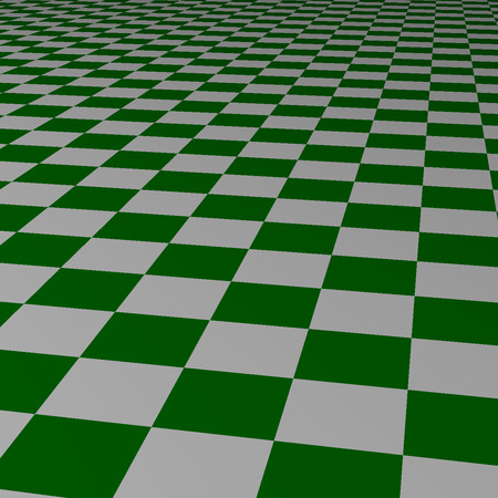
checkered-plane.yml- add: camera
  width: 400
  height: 400
  field-of-view: 0.5
  from: [1, 2, -5]
  to: [0, 0, 0]
  up: [0, 1, 0]

- add: light
  at: [-10, 10, -10]
  intensity: [1, 1, 1]

- add: plane
  material:
    pattern:
      type: map
      mapping: planar
      uv_pattern:
        type: checkers
        width: 2
        height: 2
        colors:
          - [0, 0.5, 0]
          - [1, 1, 1]
    ambient: 0.1
    specular: 0
    diffuse: 0.9
Great! Let's tackle cylinders next.
Cylindrical Mapping
The cylindrical mapping takes a pattern and wraps it around a cylinder like the label on a can of soup. Your implementation here will assume the pattern repeats every whole increment of y.
Here's a test showing how u and v map to the surface of a cylinder with a radius of 1.
patterns.featureScenario Outline: Using a cylindrical mapping on a 3D point
  Given p ← <point>
  When (u, v) ← cylindrical_map(p)
  Then u = <u>
    And v = <v>

  Examples:
    | point                          | u     | v    |
    | point(0, 0, -1)                | 0.0   | 0.0  |
    | point(0, 0.5, -1)              | 0.0   | 0.5  |
    | point(0, 1, -1)                | 0.0   | 0.0  |
    | point(0.70711, 0.5, -0.70711)  | 0.125 | 0.5  |
    | point(1, 0.5, 0)               | 0.25  | 0.5  |
    | point(0.70711, 0.5, 0.70711)   | 0.375 | 0.5  |
    | point(0, -0.25, 1)             | 0.5   | 0.75 |
    | point(-0.70711, 0.5, 0.70711)  | 0.625 | 0.5  |
    | point(-1, 1.25, 0)             | 0.75  | 0.25 |
    | point(-0.70711, 0.5, -0.70711) | 0.875 | 0.5  |
The implementation of this cylindrical_map() function will look similar to spherical_map(), at least insofar as it computes the theta angle. The y coordinate, though, maps directly to v, which is nice and tidy! Here's some pseudocode:
function cylindrical_map(p)
  # compute the azimuthal angle, same as with spherical_map()
  let theta ← arctan2(p.x, p.z)
  let raw_u ← theta / (2 * π)
  let u ← 1 - (raw_u + 0.5)

  # let v go from 0 to 1 between whole units of y
  let v ← p.y mod 1

  return (u, v)
end function
With that implemented and your tests passing, you can now render 2D patterns on the surface of a cylinder, like this:
checkered-cylinder.yml- add: camera
  width: 400
  height: 400
  field-of-view: 0.5
  from: [0, 0, -10]
  to: [0, 0, 0]
  up: [0, 1, 0]

- add: light
  at: [-10, 10, -10]
  intensity: [1, 1, 1]

- add: cylinder
  min: 0
  max: 1
  transform:
    - [translate, 0, -0.5, 0]
    - [scale, 1, 3.1415, 1]
  material:
    pattern:
      type: map
      mapping: cylindrical
      uv_pattern:
        type: checkers
        width: 16
        height: 8
        colors:
          - [0, 0.5, 0]
          - [1, 1, 1]
    ambient: 0.1
    specular: 0.6
    shininess: 15
    diffuse: 0.8
Be careful at the end-caps, though. By default, those will be textured using the same cylindrical mapping so each point will be textured based on it's y component and angle around the circle. You wind up with this look, which is probably not what you actually wanted at the poles:
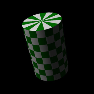
I'm not going to solve that one for you, but read on. We'll talk about cube mapping next, which may give you some ideas for how to address mapping at cylinder end caps.
Cube Mapping
Cube mapping is, unfortunately, not as straightforward as the other mappings we've looked at. The thing that makes it tricky is that instead of being a single continuous surface, a cube is actually six planar segments, and your mapping will need to take into account not only the surfaces, but how the surfaces are oriented relative to their neighbors.
That being said, cube mapping is definitely worth the effort! Later in this chapter you'll use it to implement a skybox, which lets you surround your scene in an actual photographic environment. Cube mapping is the bit that will make that all possible.
To do this, we'll start with a new UV pattern to help make sure that the sides and corners of the cube map are all aligned correctly. Once we have that pattern implemented, we'll implement a cube map that accepts six different UV patterns, one for each side of the cube.
Let's start with that new pattern.
"Align Check" Pattern
Our new pattern won't be very esthetically pleasing, but it's not meant to be. It'll just be a square of solid color, with smaller squares at the corners in different colors, like this:
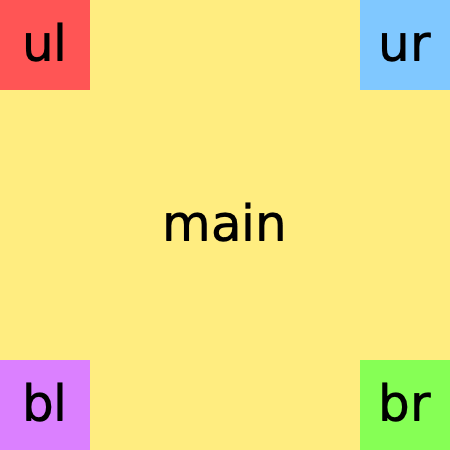
Introduce a new function, uv_align_check(main, ul, ur, bl, br), which accepts five color arguments. The main color is the primary color of the square, and ul, ur, bl, and br are the colors of the squares in (respectively) the upper left, upper right, bottom left, and bottom right.
Here's a test:
patterns.featureScenario Outline: Layout of the "align check" pattern
  Given main ← color(1, 1, 1)
    And ul ← color(1, 0, 0)
    And ur ← color(1, 1, 0)
    And bl ← color(0, 1, 0)
    And br ← color(0, 1, 1)
    And pattern ← uv_align_check(main, ul, ur, bl, br)
  When c ← uv_pattern_at(pattern, <u>, <v>)
  Then c = <expected>

  Examples:
    | u    | v    | expected |
    | 0.5  | 0.5  | main     |
    | 0.1  | 0.9  | ul       |
    | 0.9  | 0.9  | ur       |
    | 0.1  | 0.1  | bl       |
    | 0.9  | 0.1  | br       |
To implement it, check the value of u and v. If they fall within a 0.2 unit square in any of the corners of the pattern, return the corresponding color. Otherwise, return the main color. In pseudocode:
function uv_pattern_at(align_check, u, v)
  # remember: v=0 at the bottom, v=1 at the top
  if v > 0.8 then
     if u < 0.2 then return align_check.ul
     if u > 0.8 then return align_check.ur
  else if v < 0.2 then
    if u < 0.2 then return align_check.bl
    if u > 0.8 then return align_check.br
  end if

  return align_check.main
end function
Once the test is passing, feel free to verify the pattern visually; just apply it to a plane with a planar mapping, and you'll see it tiling happily away!
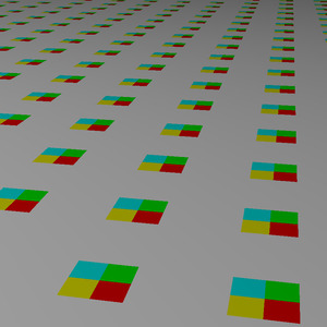
align-check-plane.yml- add: camera
  width: 400
  height: 400
  field-of-view: 0.5
  from: [1, 2, -5]
  to: [0, 0, 0]
  up: [0, 1, 0]

- add: light
  at: [-10, 10, -10]
  intensity: [1, 1, 1]

- add: plane
  material:
    pattern:
      type: map
      mapping: planar
      uv_pattern:
        type: align_check
        colors:
          main: [1, 1, 1] # white
          ul: [1, 0, 0]   # red
          ur: [1, 1, 0]   # yellow
          bl: [0, 1, 0]   # green
          br: [0, 1, 1]   # cyan
    ambient: 0.1
    diffuse: 0.8
Great! Next up: the cube mapping itself.
Implementing a Cube Mapping
Your cube mapping implementation will assume that it is mapping onto a cube with one corner at point(-1, -1, -1), and the opposite at point(1, 1, 1). It's no coincidence that this is also exactly the dimensions of the cubes in your ray tracer!
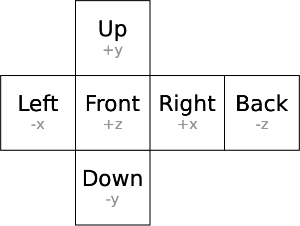
To understand how this mapping will work, let's first dissect a cube. We'll unfold it like this, in what is called a cross format. Each face is labeled with its name and corresponding axis:
The first bit you'll need, then, is a function that takes a point on a cube and tells you which face it belongs to. We'll call this function face_from_point(point). Here's a test for it:
patterns.featureScenario Outline: Identifying the face of a cube from a point
  When face ← face_from_point(<point>)
  Then face = <face>

  Examples:
    | point                  | face    |
    | point(-1, 0.5, -0.25)  | "left"  |
    | point(1.1, -0.75, 0.8) | "right" |
    | point(0.1, 0.6, 0.9)   | "front" |
    | point(-0.7, 0, -2)     | "back"  |
    | point(0.5, 1, 0.9)     | "up"    |
    | point(-0.2, -1.3, 1.1) | "down"  |
One way to implement this is to find the absolute value of each component of the point, take the highest resulting value, and then compare it against each component to determine which one must correspond to the face. This works because the coordinate with the largest absolute value will be the coordinate of the face where the point lies. In pseudocode:
function face_from_point(point)
  let abs_x ← abs(point.x)
  let abs_y ← abs(point.y)
  let abs_z ← abs(point.z)
  let coord ← max(abs_x, abs_y, abs_z)

  if coord = point.x then return "right"
  if coord = -point.x then return "left"
  if coord = point.y then return "up"
  if coord = -point.y then return "down"
  if coord = point.z then return "front"

  # the only option remaining!
  return "back"
end function
The pseudocode for face_from_point(point) returns a string, which the test also expects. In reality, this won't be a very efficient way to represent things; feel free to use symbols, integers, or whatever other scheme you feel might be more performant.
Next, you need to implement the actual mapping, taking a point on a face and converting it into a (u, v) pair. This will depend on the face that holds the point, though, so you'll implement six different functions, one for each face of the cube. Here are six scenarios that demonstrate the desired behavior of each of these functions.
patterns.featureScenario Outline: UV mapping the front face of a cube
  When (u, v) ← cube_uv_front(<point>)
  Then u = <u>
    And v = <v>

  Examples:
    | point                | u    | v    |
    | point(-0.5, 0.5, 1)  | 0.25 | 0.75 |
    | point(0.5, -0.5, 1)  | 0.75 | 0.25 |

Scenario Outline: UV mapping the back face of a cube
  When (u, v) ← cube_uv_back(<point>)
  Then u = <u>
    And v = <v>

  Examples:
    | point                 | u    | v    |
    | point(0.5, 0.5, -1)   | 0.25 | 0.75 |
    | point(-0.5, -0.5, -1) | 0.75 | 0.25 |

Scenario Outline: UV mapping the left face of a cube
  When (u, v) ← cube_uv_left(<point>)
  Then u = <u>
    And v = <v>

  Examples:
    | point                | u    | v    |
    | point(-1, 0.5, -0.5) | 0.25 | 0.75 |
    | point(-1, -0.5, 0.5) | 0.75 | 0.25 |

Scenario Outline: UV mapping the right face of a cube
  When (u, v) ← cube_uv_right(<point>)
  Then u = <u>
    And v = <v>

  Examples:
    | point                | u    | v    |
    | point(1, 0.5, 0.5)   | 0.25 | 0.75 |
    | point(1, -0.5, -0.5) | 0.75 | 0.25 |

Scenario Outline: UV mapping the upper face of a cube
  When (u, v) ← cube_uv_up(<point>)
  Then u = <u>
    And v = <v>

  Examples:
    | point               | u    | v    |
    | point(-0.5, 1, -0.5) | 0.25 | 0.75 |
    | point(0.5, 1, 0.5) | 0.75 | 0.25 |

Scenario Outline: UV mapping the lower face of a cube
  When (u, v) ← cube_uv_down(<point>)
  Then u = <u>
    And v = <v>

  Examples:
    | point                 | u    | v    |
    | point(-0.5, -1, 0.5) | 0.25 | 0.75 |
    | point(0.5, -1, -0.5)   | 0.75 | 0.25 |
To understand how these ought to be implemented, let's start by looking at just the cube_uv_front(point) function. The following diagram shows how the front of the cube is treated by this function:
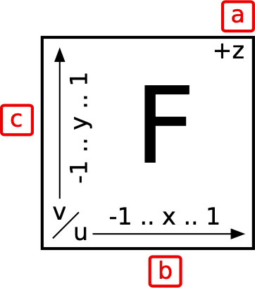
The +z in the upper right (at a) indicates the axis with which the face is aligned, and the arrows at b and c show how the axes map to u and v. In this case, u goes from 0 to 1 as x goes from -1 to 1, and v goes from 0 to 1 as y goes from -1 to 1.
Great! With a bit of mental gymnastics, we can see that to get u from x, we:
- Add 1 to
x, adjusting the range to 0..2, - Modulo the result by 2, so that points outside that range will repeat, and
- Divide that by 2, so the final range is 0..1.
This is the same for getting v from y. The cube_uv_front(point) function will look something like this, then, in pseudocode:
function cube_uv_front(point)
  let u ← ((point.x + 1) mod 2.0) / 2.0
  let v ← ((point.y + 1) mod 2.0) / 2.0

  return (u, v)
end
Now, let's look at the back face of the cube. Here's its diagram:
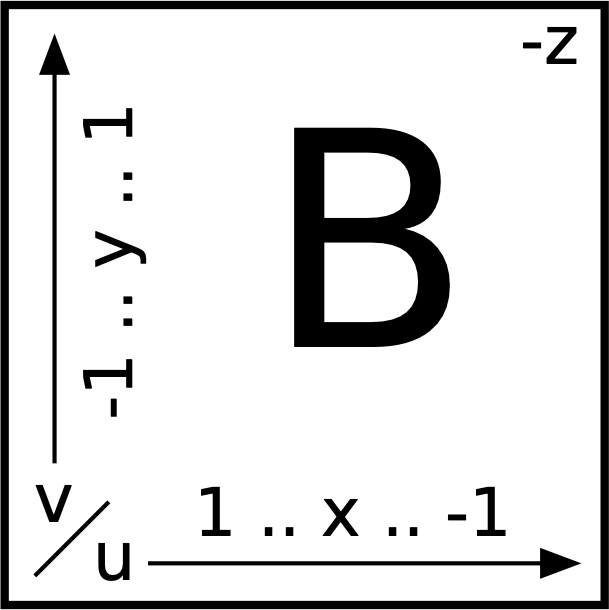
Once again, v goes from 0 to 1 as y goes from -1 to 1, but the u mapping is backward now, going from 0 to 1 as x goes downward from 1 to -1. That is to say, 1 must map to 0, and -1 must map to 1. Our algorithm remains nearly the same, but now we subtract x from 1, instead of adding. Here's the pseudocode for cube_uv_back(point)
function cube_uv_back(point)
  let u ← ((1 - point.x) mod 2.0) / 2.0
  let v ← ((point.y + 1) mod 2.0) / 2.0

  return (u, v)
end
Only four more to go! However, instead of handing you the pseudocode for each of them in turn, I'm going to give you a diagram showing all of the cube's faces, and let you work out the remaining four functions. Here's the diagram:
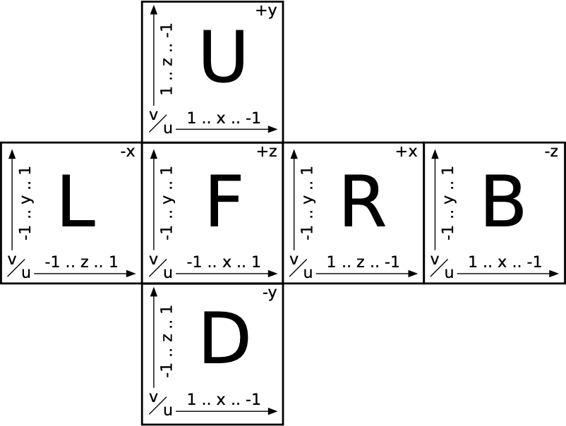
(click to enlarge)
Use the cube_uv_front() and cube_uv_back() functions as templates, and make the remaining mappings work. You've got this!
Once those functions are all passing, there's just one piece remaining: you need to implement a CubeMap subclass of Pattern, and the corresponding version of pattern_at(cube_map, point).
The CubeMap subclass must encapsulate a collection of six uv_pattern instances, one for each face. The following (rather lengthy!) test uses the uv_align_check() pattern for each face, and tests that the corners and middles are all being evaluated as expected.
patterns.featureScenario Outline: Finding the colors on a mapped cube
  When red ← color(1, 0, 0)
    And yellow ← color(1, 1, 0)
    And brown ← color(1, 0.5, 0)
    And green ← color(0, 1, 0)
    And cyan ← color(0, 1, 1)
    And blue ← color(0, 0, 1)
    And purple ← color(1, 0, 1)
    And white ← color(1, 1, 1)
    And left ← uv_align_check(yellow, cyan, red, blue, brown)
    And front ← uv_align_check(cyan, red, yellow, brown, green)
    And right ← uv_align_check(red, yellow, purple, green, white)
    And back ← uv_align_check(green, purple, cyan, white, blue)
    And up ← uv_align_check(brown, cyan, purple, red, yellow)
    And down ← uv_align_check(purple, brown, green, blue, white)
    And pattern ← cube_map(left, front, right, back, up, down)
  Then pattern_at(pattern, <point>) = <color>

  Examples:
    |   | point                 | color  |
    | L | point(-1, 0, 0)       | yellow |
    |   | point(-1, 0.9, -0.9)  | cyan   |
    |   | point(-1, 0.9, 0.9)   | red    |
    |   | point(-1, -0.9, -0.9) | blue   |
    |   | point(-1, -0.9, 0.9)  | brown  |
    | F | point(0, 0, 1)        | cyan   |
    |   | point(-0.9, 0.9, 1)   | red    |
    |   | point(0.9, 0.9, 1)    | yellow |
    |   | point(-0.9, -0.9, 1)  | brown  |
    |   | point(0.9, -0.9, 1)   | green  |
    | R | point(1, 0, 0)        | red    |
    |   | point(1, 0.9, 0.9)    | yellow |
    |   | point(1, 0.9, -0.9)   | purple |
    |   | point(1, -0.9, 0.9)   | green  |
    |   | point(1, -0.9, -0.9)  | white  |
    | B | point(0, 0, -1)       | green  |
    |   | point(0.9, 0.9, -1)   | purple |
    |   | point(-0.9, 0.9, -1)  | cyan   |
    |   | point(0.9, -0.9, -1)  | white  |
    |   | point(-0.9, -0.9, -1) | blue   |
    | U | point(0, 1, 0)        | brown  |
    |   | point(-0.9, 1, -0.9)  | cyan   |
    |   | point(0.9, 1, -0.9)   | purple |
    |   | point(-0.9, 1, 0.9)   | red    |
    |   | point(0.9, 1, 0.9)    | yellow |
    | D | point(0, -1, 0)       | purple |
    |   | point(-0.9, -1, 0.9)  | brown  |
    |   | point(0.9, -1, 0.9)   | green  |
    |   | point(-0.9, -1, -0.9) | blue   |
    |   | point(0.9, -1, -0.9)  | white  |
To make this real, your cube map's pattern_at() function needs to first use face_from_point() to figure out which face the point lies on, and then call the corresponding cube_uv_<face>() function to get the u and v values. Once you've got those, you can query the face's uv_pattern to get the final color value. In pseudocode:
function pattern_at(cube_map, point)
  let face ← face_from_point(point)

  if face = "left" then
    (u, v) ← uv_cube_left(point)
  else if face = "right" then
    (u, v) ← uv_cube_right(point)
  else if face = "front" then
    (u, v) ← uv_cube_front(point)
  else if face = "back" then
    (u, v) ← uv_cube_back(point)
  else if face = "up" then
    (u, v) ← uv_cube_up(point)
  else # down
    (u, v) ← uv_cube_down(point)
  end

  return uv_pattern_at(cube_map.faces[face], u, v)
end
Once all your tests are passing, try rendering the cube from that last test and seeing how it looks. Care has been taken to ensure that the textures at each corner are the same on each adjacent face; that is to say, if one face declares a corner to be red, the other two faces at that corner also declare that corner to be red. This means that if you rotate it to inspect each corner, you'll see each corner appears to be a solid block, like this:
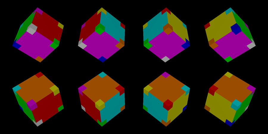
checkered-cube.yml- add: camera
  width: 800
  height: 400
  field-of-view: 0.8
  from: [0, 0, -20]
  to: [0, 0, 0]
  up: [0, 1, 0]

- add: light
  at: [0, 100, -100]
  intensity: [0.25, 0.25, 0.25]
- add: light
  at: [0, -100, -100]
  intensity: [0.25, 0.25, 0.25]
- add: light
  at: [-100, 0, -100]
  intensity: [0.25, 0.25, 0.25]
- add: light
  at: [100, 0, -100]
  intensity: [0.25, 0.25, 0.25]

- define: MappedCube
  value:
    add: cube
    material:
      pattern:
        type: map
        mapping: cube
        left:
          type: align_check
          colors:
            main: [1, 1, 0] # yellow
            ul: [0, 1, 1]   # cyan
            ur: [1, 0, 0]   # red
            bl: [0, 0, 1]   # blue
            br: [1, 0.5, 0] # brown
        front:
          type: align_check
          colors:
            main: [0, 1, 1] # cyan
            ul: [1, 0, 0]   # red
            ur: [1, 1, 0]   # yellow
            bl: [1, 0.5, 0] # brown
            br: [0, 1, 0]   # green
        right:
          type: align_check
          colors:
            main: [1, 0, 0] # red
            ul: [1, 1, 0]   # yellow
            ur: [1, 0, 1]   # purple
            bl: [0, 1, 0]   # green
            br: [1, 1, 1]   # white
        back:
          type: align_check
          colors:
            main: [0, 1, 0] # green
            ul: [1, 0, 1]   # purple
            ur: [0, 1, 1]   # cyan
            bl: [1, 1, 1]   # white
            br: [0, 0, 1]   # blue
        up:
          type: align_check
          colors:
            main: [1, 0.5, 0] # brown
            ul: [0, 1, 1]   # cyan
            ur: [1, 0, 1]   # purple
            bl: [1, 0, 0]   # red
            br: [1, 1, 0]   # yellow
        down:
          type: align_check
          colors:
            main: [1, 0, 1] # purple
            ul: [1, 0.5, 0] # brown
            ur: [0, 1, 0]   # green
            bl: [0, 0, 1]   # blue
            br: [1, 1, 1]   # white
      ambient: 0.2
      specular: 0
      diffuse: 0.8

- add: MappedCube
  transform:
    - [rotate-y, 0.7854]
    - [rotate-x, 0.7854]
    - [translate, -6, 2, 0]

- add: MappedCube
  transform:
    - [rotate-y, 2.3562]
    - [rotate-x, 0.7854]
    - [translate, -2, 2, 0]

- add: MappedCube
  transform:
    - [rotate-y, 3.927]
    - [rotate-x, 0.7854]
    - [translate, 2, 2, 0]

- add: MappedCube
  transform:
    - [rotate-y, 5.4978]
    - [rotate-x, 0.7854]
    - [translate, 6, 2, 0]

- add: MappedCube
  transform:
    - [rotate-y, 0.7854]
    - [rotate-x, -0.7854]
    - [translate, -6, -2, 0]

- add: MappedCube
  transform:
    - [rotate-y, 2.3562]
    - [rotate-x, -0.7854]
    - [translate, -2, -2, 0]

- add: MappedCube
  transform:
    - [rotate-y, 3.927]
    - [rotate-x, -0.7854]
    - [translate, 2, -2, 0]

- add: MappedCube
  transform:
    - [rotate-y, 5.4978]
    - [rotate-x, -0.7854]
    - [translate, 6, -2, 0]
Having those corners all matched up like that is important—it means you can create cube map textures that seamlessly wrap from one face to another. This will be especially critical in skyboxes, but before we can get to that, we need one more intermediate step: image mapping.
Image Mapping
Image mapping is the name of a technique that lets you use image data to texture objects in your scene. Perhaps you're taking an actual image of a soup can label and wrapping it around a cylinder, or taking a map of Earth or the Moon and putting it on a sphere. The primary benefit it affords is that you can create a super realistic-looking environment with very little effort.
Before you can map images to your objects, though, you first need to be able to load image data into memory. If you'd like, please feel free to skip the next subsection and take advantage of existing libraries, like libpng or libjpeg, or whatever other library you prefer for reading and parsing common image file formats.
For those who don't want to wrangle those API's, or who (like me) find something satisfying about writing things from scratch, read on! The first part of this section will involve adding to your canvas implementation (from chapter 2 of The Ray Tracer Challenge), and making it support not only writing PPM files, but reading them, too. This way, you can use a tool like ImageMagick to take any image you like and convert it to PPM, and then load it straight into your scenes.
Reading a PPM image into a canvas
Just as with your PPM writer, your PPM reader is only going to support PPM files of type "P3", which are those that are in plain text format. We'll tackle this in a few tests.
To start, you need to make sure that your PPM reader only accepts files that start with the magic number "P3", followed by a newline. The following test introduces a new function, canvas_from_ppm(file), which will (eventually) parse the given PPM-formatted file and return a new canvas. In this test, it is given a file with a bad magic number, which should fail.
canvas.featureScenario: Reading a file with the wrong magic number
  Given ppm ← a file containing:
    """
    P32
    1 1
    255
    0 0 0
    """
  Then canvas_from_ppm(ppm) should fail
The actual meaning of "should fail" is up to you! If your programming language supports exceptions, perhaps your canvas_from_ppm() function can raise an exception in this case. Otherwise, maybe it returns a null value, or sets some global variable to assert that an error occured (like C does with its errno variable).
Once you've got that far, the next step is to make sure that the returned canvas is of the correct dimensions. As you'll recall from chapter 2, "Drawing on a Canvas", the two numbers on the line immediately after the magic number identify the width and height of the image. The following test makes sure the canvas matches the expected size.
canvas.featureScenario: Reading a PPM returns a canvas of the right size
  Given ppm ← a file containing:
    """
    P3
    10 2
    255
    0 0 0  0 0 0  0 0 0  0 0 0  0 0 0
    0 0 0  0 0 0  0 0 0  0 0 0  0 0 0
    0 0 0  0 0 0  0 0 0  0 0 0  0 0 0
    0 0 0  0 0 0  0 0 0  0 0 0  0 0 0
    """
  When canvas ← canvas_from_ppm(ppm)
  Then canvas.width = 10
    And canvas.height = 2
Nice! Next, you need to make sure your reader actually parses the pixel data correctly.
Recall that the third line is the scale of the colors, or the maximum value that any component may take. In the following test, the scale is 255. You'll want to divide each color component by that value to convert them into a floating point number between 0 and 1.
After that, subsequent lines are triples of integers representing consecutive red, green, and blue values. Every set of three numbers corresponds to a single pixel, and the pixel positions increase in x first, then y.
The following test checks every pixel of a (small) image to make sure that your reader has parsed them correctly and placed them at the correct position in the canvas.
canvas.featureScenario Outline: Reading pixel data from a PPM file
  Given ppm ← a file containing:
    """
    P3
    4 3
    255
    255 127 0  0 127 255  127 255 0  255 255 255
    0 0 0  255 0 0  0 255 0  0 0 255
    255 255 0  0 255 255  255 0 255  127 127 127
    """
  When canvas ← canvas_from_ppm(ppm)
  Then pixel_at(canvas, <x>, <y>) = <color>

  Examples:
    | x | y | color                      |
    | 0 | 0 | color(1, 0.498, 0)         |
    | 1 | 0 | color(0, 0.498, 1)         |
    | 2 | 0 | color(0.498, 1, 0)         |
    | 3 | 0 | color(1, 1, 1)             |
    | 0 | 1 | color(0, 0, 0)             |
    | 1 | 1 | color(1, 0, 0)             |
    | 2 | 1 | color(0, 1, 0)             |
    | 3 | 1 | color(0, 0, 1)             |
    | 0 | 2 | color(1, 1, 0)             |
    | 1 | 2 | color(0, 1, 1)             |
    | 2 | 2 | color(1, 0, 1)             |
    | 3 | 2 | color(0.498, 0.498, 0.498) |
Make that pass, and then there's a kind of annoying case that you ought to be able to handle. Some tools (like ImageMagick) have a tendency to insert comments into the PPM files they produce, which will bite you if you don't handle them correctly. Fortunately, comments are easy to detect: they're always preceded by a # character, and you can assume they always occupy an entire line, like in this test:
canvas.featureScenario: PPM parsing ignores comment lines
  Given ppm ← a file containing:
    """
    P3
    # this is a comment
    2 1
    # this, too
    255
    # another comment
    255 255 255
    # oh, no, comments in the pixel data!
    255 0 255
    """
  When canvas ← canvas_from_ppm(ppm)
  Then pixel_at(canvas, 0, 0) = color(1, 1, 1)
    And pixel_at(canvas, 1, 0) = color(1, 0, 1)
There are just two final edge cases that your parser ought to handle. The first is that a single RGB triple might be broken by a new line, and your parser needs to be able to silently skip over those line breaks. The following test provides a one-pixel PPM file, where each component of that pixel is followed by a newline character.
canvas.featureScenario: PPM parsing allows an RGB triple to span lines
  Given ppm ← a file containing:
    """
    P3
    1 1
    255
    51
    153

    204
    """
  When canvas ← canvas_from_ppm(ppm)
  Then pixel_at(canvas, 0, 0) = color(0.2, 0.6, 0.8)
There will, of course, be many ways to implement this. If you're at a loss, you might consider creating a separate abstraction for extracting integers from an IO stream. The abstraction doesn't worry about RGB triples or any of that, just pulling consecutive integers out of the stream, and can thus look for and skip over newlines (and comments!) in the stream.
You probably already have the last special case working. The following test just makes sure that your parser handles different scale values, by giving you a file where the maximum component value is 100.
canvas.featureScenario: PPM parsing respects the scale setting
  Given ppm ← a file containing:
    """
    P3
    2 2
    100
    100 100 100  50 50 50
    75 50 25  0 0 0
    """
  When canvas ← canvas_from_ppm(ppm)
  Then pixel_at(canvas, 0, 1) = color(0.75, 0.5, 0.25)
There! When those tests are all passing, you're ready for the next phase: producing an actual image map.
Making an Image-Based UV Pattern
So far, your UV patterns (checkers and align-check) have been programmatic, and geometrical, relying on math to determine the color at a given (u, v) coordinate. What you're going to do in this section is create a new UV pattern that maps a (u, v) coordinate to a pixel in an image.
Here's a test that provides a PPM file containing a grayscale gradient, and then introduces a new function, uv_image(canvas), which accepts a canvas instance and returns a new UV pattern that encapsulates it. The test shows how asking for the color at a given (u, v) location returns the corresponding color from the canvas.
patterns.featureScenario Outline: Checker pattern in 2D
  Given ppm ← a file containing:
    """
    P3
    10 10
    10
    0 0 0  1 1 1  2 2 2  3 3 3  4 4 4  5 5 5  6 6 6  7 7 7  8 8 8  9 9 9
    1 1 1  2 2 2  3 3 3  4 4 4  5 5 5  6 6 6  7 7 7  8 8 8  9 9 9  0 0 0
    2 2 2  3 3 3  4 4 4  5 5 5  6 6 6  7 7 7  8 8 8  9 9 9  0 0 0  1 1 1
    3 3 3  4 4 4  5 5 5  6 6 6  7 7 7  8 8 8  9 9 9  0 0 0  1 1 1  2 2 2
    4 4 4  5 5 5  6 6 6  7 7 7  8 8 8  9 9 9  0 0 0  1 1 1  2 2 2  3 3 3
    5 5 5  6 6 6  7 7 7  8 8 8  9 9 9  0 0 0  1 1 1  2 2 2  3 3 3  4 4 4
    6 6 6  7 7 7  8 8 8  9 9 9  0 0 0  1 1 1  2 2 2  3 3 3  4 4 4  5 5 5
    7 7 7  8 8 8  9 9 9  0 0 0  1 1 1  2 2 2  3 3 3  4 4 4  5 5 5  6 6 6
    8 8 8  9 9 9  0 0 0  1 1 1  2 2 2  3 3 3  4 4 4  5 5 5  6 6 6  7 7 7
    9 9 9  0 0 0  1 1 1  2 2 2  3 3 3  4 4 4  5 5 5  6 6 6  7 7 7  8 8 8
    """
    And canvas ← canvas_from_ppm(ppm)
    And pattern ← uv_image(canvas)
  When color ← uv_pattern_at(pattern, <u>, <v>)
  Then color = <expected>

  Examples:
    | u   | v   | expected             |
    | 0   | 0   | color(0.9, 0.9, 0.9) |
    | 0.3 | 0   | color(0.2, 0.2, 0.2) |
    | 0.6 | 0.3 | color(0.1, 0.1, 0.1) |
    | 1   | 1   | color(0.9, 0.9, 0.9) |
There are two "gotchas" to keep in mind when implementing this. First, make sure you multiply u and v by width - 1 and height - 1, instead of the full width and height, so that you don't overflow your canvas when u or v are 1. Second, you need to flip v around, since your UV mapping treats the bottom as v=0, but your canvas treats the top as y=0.
In pseudocode, your uv_pattern_at() function for a UV image will look something like this:
function uv_pattern_at(uv_image, u, v)
  # flip v over so it matches the image layout, with y at the top
  let v ← 1 - v

  let x ← u * (uv_image.canvas.width - 1)
  let y ← v * (uv_image.canvas.height - 1)

  # be sure and round x and y to the nearest whole number
  return pixel_at(uv_image.canvas, round(x), round(y))
end function
Assuming your tests are all passing, you should now be able to render an image-mapped sphere, like this one:
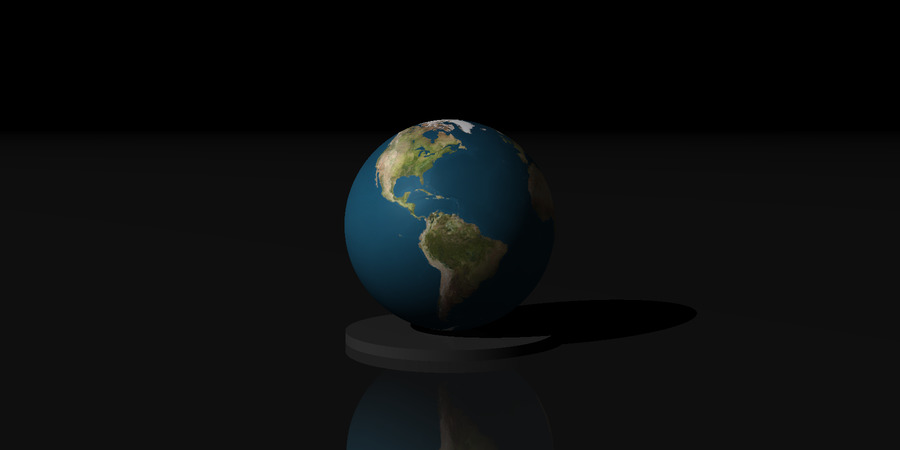
earth.yml- add: camera
  width: 800
  height: 400
  field-of-view: 0.8
  from: [1, 2, -10]
  to: [0, 1.1, 0]
  up: [0, 1, 0]

- add: light
  at: [-100, 100, -100]
  intensity: [1, 1, 1]

- add: plane
  material:
    color: [1, 1, 1]
    diffuse: 0.1
    specular: 0
    ambient: 0
    reflective: 0.4

- add: cylinder
  min: 0
  max: 0.1
  closed: true
  material:
    color: [1, 1, 1]
    diffuse: 0.2
    specular: 0
    ambient: 0
    reflective: 0.1

# the earth image map is from
# http://planetpixelemporium.com/earth.html (see "color map")
#
# converted from JPG to PPM via ImageMagick with:
# $ convert earthmap1k.jpg -compress none earthmap1k.ppm

- add: sphere
  transform:
    - [ rotate-y, 1.9 ]
    - [ translate, 0, 1.1, 0 ]
  material:
    pattern:
      type: map
      mapping: spherical
      uv_pattern:
        type: image
        file: earthmap1k.ppm
    diffuse: 0.9
    specular: 0.1
    shininess: 10
    ambient: 0.1
There are no doubt a variety of ways to convert an image to PPM "P3" format. My personal favorite is to use ImageMagick's convert tool. To convert image.jpg to image.ppm, you'd use the following invocation:
$ convert image.jpg -compress none image.ppm
Specifying -compress none ensures the result is a plain text, "P3"-formatted PPM file.
Excellent! Let's look at one last thing before we wrap up this chapter: skyboxes.
Skyboxes
What is a skybox? It's just a cube that has been textured with six images, where the images form a seamless immersive environment. There are many places online where you can get skybox imagery, either for a fee or for free. For example, Humus has a beautiful collection of a variety of environments that he's made available under a CC BY 3.0 license.
Skyboxes come in several formats. For your purposes, based on the implementation described in this chapter, you want to find skyboxes that are distributed as six square images, typically labeled as "posx", "negz", etc. Alternatively, you'll find them distributed in cross format, which is a single image where the skybox itself is laid out in an exploded cube, like the diagrams in this chapter. I leave it as an exercise for you to figure out how to support such formats directly!
Alternatively, you can create a sky "box" using a sphere, as well. This is appropriate if the image you want to use as the environment is provided as a spherical mapping, instead of a cube mapping. One site with quite a few beautiful spherically mapped images of this sort is HDRI Haven.
Once you've got your skybox images, you construct the actual skybox like so:
- Add a cube (or sphere) to your scene.
- Apply a cube map (or, if using a sphere, a spherical map) to it, with the skybox images in the correct order.
- Scale the cube or sphere so it is very large. The other objects in your scene must never interact with the skybox, or it will ruin the illusion.
- Set the
ambientvalue to 1, andspecularanddiffuseto 0. You do not want the skybox to interact with light sources at all, to preserve the illusion.
Though not strictly necessary, it's also a very good idea to make sure that the light sources in your scene roughly correspond to any light sources in the skybox, so that lighting and shadows don't contradict what the skybox is doing. For example, if the sun is directly overhead in the skybox, you'll want to put a light source directly overhead in your scene, as well.
Here's a simple image consisting solely of a skybox and a small reflective sphere, to give you some idea of how convincing it can be:
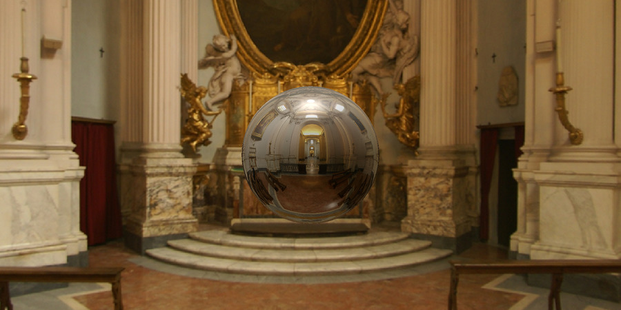
skybox.yml- add: camera
  width: 800
  height: 400
  field-of-view: 1.2
  from: [0, 0, 0]
  to: [0, 0, 5]
  up: [0, 1, 0]

- add: light
  at: [0, 100, 0]
  intensity: [1, 1, 1]

- add: sphere
  transform:
    - [ scale, 0.75, 0.75, 0.75 ]
    - [ translate, 0, 0, 5 ]
  material:
    diffuse: 0.4
    specular: 0.6
    shininess: 20
    reflective: 0.6
    ambient: 0

# the cube map image is from Lancellotti Chapel from
# http://www.humus.name/index.php?page=Textures

- add: cube
  transform:
    - [ scale, 1000, 1000, 1000 ]
  material:
    pattern:
      type: map
      mapping: cube
      left:
        type: image
        file: negx.ppm
      right:
        type: image
        file: posx.ppm
      front:
        type: image
        file: posz.ppm
      back:
        type: image
        file: negz.ppm
      up:
        type: image
        file: posy.ppm
      down:
        type: image
        file: negy.ppm
    diffuse: 0
    specular: 0
    ambient: 1
Not bad, for a scene of just two objects!
Wrapping it up
And that's texture mapping in a nutshell! Looking back over the chapter, I guess it was a rather large nutshell. You don't have to dig very deep to discover that this rabbit hole goes way down.
Here are some other things you might want to experiment with, related to texture maps and image maps:
- If your image maps are small-ish, you may find the resulting textures look blocky and pixelated. The best solution to this is to use higher resolution images, but a nice compromise is to implement bilinear interpolation. This averages the colors of adjacent pixels in the image and can produce a smoother result in some situations.
- Contrariwise, if your image maps are very high resolution, you'll find that the objects might look noisy, laced with static. Sampling your objects at a higher resolution (like you'd do to antialias your images) can help with this greatly. In a pinch, you can render the entire scene at 2 or 3 times the resolution you need, and then resize them smaller, but that's wasteful when all you really need is to supersample the image-mapped objects. How might you go about supersampling just certain objects in your scene? There's a puzzle for you!
- If you've gotten through chapter 15, "Triangles", then you've implemented an OBJ file parser. The OBJ file format has a complementary file format called MTL ("material"), which describes how an object can be textured. You can read more about it here: http://www.fileformat.info/format/material/. How might you implement this file format so that your OBJ models can be textured and colored as originally envisioned by the models' authors?
Even if you go no farther than what was implemented in this chapter, you'll still have plenty to keep you busy. Experiment and see what you come up. Most important of all: have fun!
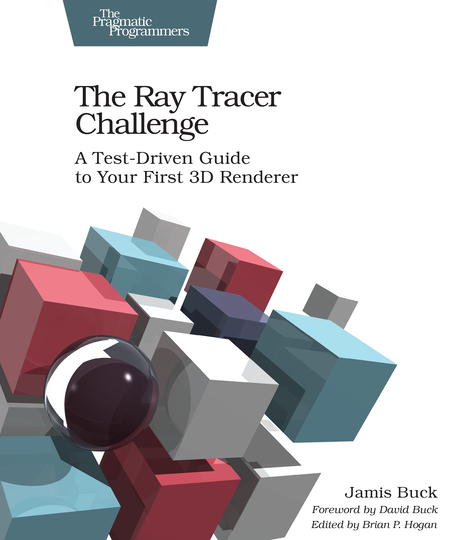
Did you like what you read here? The book follows the same format! With extensive tests and pseudocode, it will walk you through writing a ray tracer of your very own, from scratch. Grab your copy today!
If you've already purchased my book: thank you, thank you, thank you! I hope you find the same satisfaction I've found in writing your own 3D renderer.
Reviews really do drive sales, though, so it would mean a lot to me if you could leave a review of the book somewhere: Amazon.com, Goodreads.com, Twitter, Facebook, your own personal website, or any other place where folks might come across your review.
Thanks!
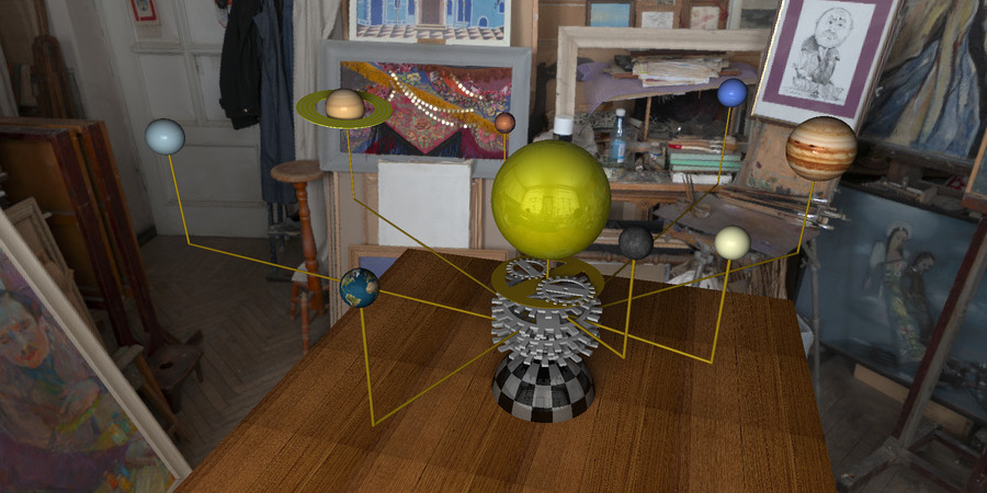
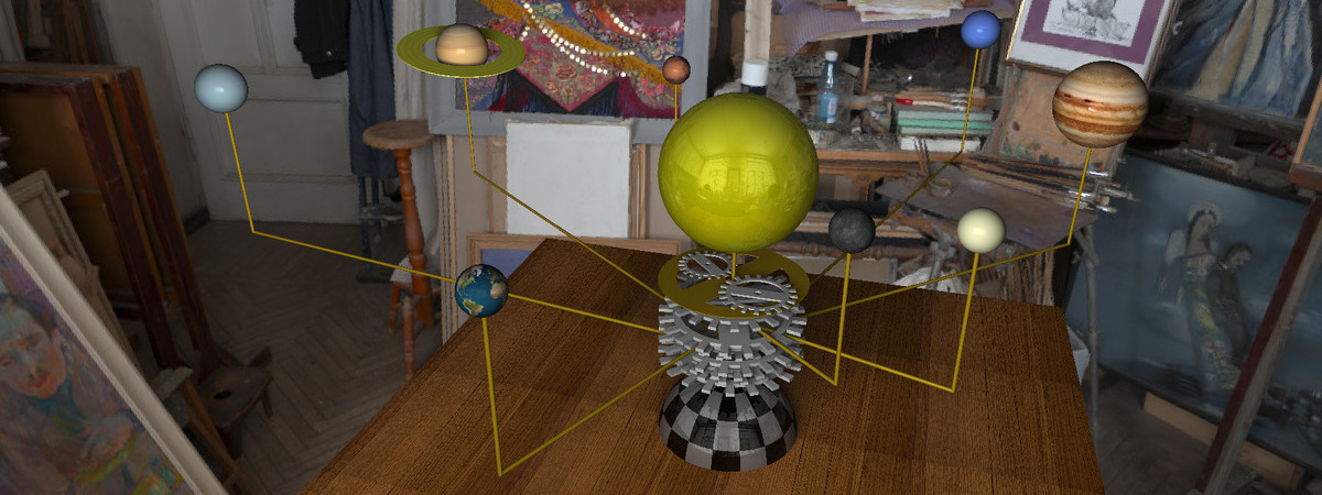
orrery.yml# ======================================================
# orrery.yml
#
# This file describes the title image for the "Texture
# Mapping" bonus chapter at:
#
# http://www.raytracerchallenge.com/bonus/texture-mapping.html
#
# It requires several additional resources, provided as a
# separate download. The resources were found on the following
# sites:
#
# * https://www.bittbox.com/freebies/free-hi-resolution-wood-textures
#   : the wooden texture for the table
# * https://astrogeology.usgs.gov/search/map/Mercury/Messenger/Global/Mercury_MESSENGER_MDIS_Basemap_LOI_Mosaic_Global_166m
#   : the map of Mercury
# * http://planetpixelemporium.com/planets.html
#   : maps of Earth, Mars, Jupiter, Saturn, Uranus, and Neptune
# * https://hdrihaven.com/hdri/?c=indoor&h=artist_workshop
#   : the "artist workshop" environment map
#
# by Jamis Buck <jamis@jamisbuck.org>
# ======================================================

- add: camera
  width: 800
  height: 400
  field-of-view: 1.2
  from: [2, 4, -10]
  to: [-1, -1, 0]
  up: [0, 1, 0]

# The scene as shown in the bonus chapter is rendered using an area light,
# precisely as described in the "Rendering soft shadows" bonus chapter,
# here: http://www.raytracerchallenge.com/bonus/area-light.html
#
# if you haven't implemented area lights, you can replace this with a point
# light located at [0, 2.5, -10].

- add: light
  corner: [-5, 0, -10]
  uvec: [10, 0, 0]
  vvec: [0, 5, 0]
  usteps: 10
  vsteps: 5
  jitter: true
  intensity: [1, 1, 1]

# -------------------------------------------
# some common textures
# -------------------------------------------

- define: GOLD
  value:
    color: [ 1, 0.8, 0.1 ]
    ambient: 0.1
    diffuse: 0.6
    specular: 0.3
    shininess: 15

- define: SILVER
  value:
    color: [ 1, 1, 1 ]
    ambient: 0.1
    diffuse: 0.7
    specular: 0.3
    shininess: 15

# -----------------------------------------------
# CSG definition for the gears used to construct
# the orrery.
#
# NOTCH is a helper object used to create the
# teeth for the gears.
#
# GEAR is the actual gear object itself.
# -----------------------------------------------

- define: NOTCH
  value:
    add: csg
    operation: difference
    left:
      type: cube
      transform:
        - [ scale, 1, 0.25, 1 ]
        - [ translate, 1, 0, 1 ]
        - [ rotate-y, 0.7854 ]
        - [ scale, 1, 1, 0.1 ]
    right:
      type: cylinder
      min: -0.26
      max: 0.26
      closed: true
      transform:
        - [ scale, 0.8, 1, 0.8 ]

- define: GEAR
  value:
    add: csg
    operation: difference
    left:
      type: cylinder
      min: -0.025
      max: 0.025
      closed: true
    right:
      type: group
      children:
        # center hole
        - add: cylinder
          min: -0.06
          max: 0.06
          closed: true
          transform:
            - [ scale, 0.1, 1, 0.1 ]
        # crescents
        - add: csg
          operation: difference
          left:
            type: cylinder
            min: -0.06
            max: 0.06
            closed: true
            transform:
              - [ scale, 0.7, 1, 0.7 ]
          right:
            type: cube
            transform:
              - [ scale, 1, 0.1, 0.2 ]
        # teeth
        - add: NOTCH
        - add: NOTCH
          transform:
            - [ rotate-y, 0.31415 ]
        - add: NOTCH
          transform:
            - [ rotate-y, 0.6283 ]
        - add: NOTCH
          transform:
            - [ rotate-y, 0.94245 ]
        - add: NOTCH
          transform:
            - [ rotate-y, 1.2566 ]
        - add: NOTCH
          transform:
            - [ rotate-y, 1.57075 ]
        - add: NOTCH
          transform:
            - [ rotate-y, 1.8849 ]
        - add: NOTCH
          transform:
            - [ rotate-y, 2.19905 ]
        - add: NOTCH
          transform:
            - [ rotate-y, 2.5132 ]
        - add: NOTCH
          transform:
            - [ rotate-y, 2.82735 ]
        - add: NOTCH
          transform:
            - [ rotate-y, 3.1415 ]
        - add: NOTCH
          transform:
            - [ rotate-y, -0.31415 ]
        - add: NOTCH
          transform:
            - [ rotate-y, -0.6283 ]
        - add: NOTCH
          transform:
            - [ rotate-y, -0.94245 ]
        - add: NOTCH
          transform:
            - [ rotate-y, -1.2566 ]
        - add: NOTCH
          transform:
            - [ rotate-y, -1.57075 ]
        - add: NOTCH
          transform:
            - [ rotate-y, -1.8849 ]
        - add: NOTCH
          transform:
            - [ rotate-y, -2.19905 ]
        - add: NOTCH
          transform:
            - [ rotate-y, -2.5132 ]
        - add: NOTCH
          transform:
            - [ rotate-y, -2.82735 ]

# mechanism: top plate
- add: csg
  operation: difference
  material: GOLD
  transform:
    - [ rotate-y, -1 ]
  left:
    type: cylinder
    min: -1.51
    max: -1.5
    closed: true
  right:
    type: group
    children:
      - add: cylinder
        min: -1.52
        max: -1.49
        closed: true
        transform:
          - [ scale, 0.1, 1, 0.1 ]
      - add: csg
        operation: difference
        left:
          type: cylinder
          min: -1.52
          max: -1.49
          closed: true
          transform:
            - [ scale, 0.75, 1, 0.75 ]
        right:
          type: cube
          transform:
            - [ scale, 1, 0.1, 0.2 ]
            - [ translate, 0, -1.5, 0 ]

# mechanism: gear
- add: GEAR
  material: SILVER
  transform:
    - [ scale, 0.5, 0.5, 0.5 ]
    - [ translate, 0.4, -1.45, -0.4 ]

# mechanism: gear
- add: GEAR
  material: SILVER
  transform:
    - [ rotate-y, 0.8 ]
    - [ scale, 0.4, 0.4, 0.4 ]
    - [ translate, -0.4, -1.45, 0.2 ]

# sun
- add: group
  children:
    - add: sphere
      shadow: false
      material:
        color: [1, 1, 0]
        ambient: 0.1
        diffuse: 0.6
        specular: 0 # count on the skybox reflection being the specular highlight
        reflective: 0.2
    - add: group
      material: GOLD
      children:
        - add: cylinder
          min: -4
          max: -0.5
          transform:
            - [ scale, 0.025, 1, 0.025 ]

# base
- add: sphere
  transform:
    - [ translate, 0, -4, 0 ]
  material:
    pattern:
      type: map
      mapping: spherical
      uv_pattern:
        type: checkers
        width: 16
        height: 8
        colors:
          - [ 0, 0, 0 ]
          - [ 0.5, 0.5, 0.5 ]
    diffuse: 0.6
    specular: 0 # count on the skybox reflection being the specular highlight
    ambient: 0.1
    reflective: 0.2

# table
- add: cube
  transform:
    - [ scale, 5, 0.1, 5 ]
    - [ translate, 0, -4, 0 ]
  material:
    diffuse: 0.9
    ambient: 0.1
    specular: 0
    pattern:
      type: map
      mapping: planar
      uv_pattern:
        type: image
        file: res/wood.ppm
      transform:
        - [ scale, 0.5, 0.5, 0.5 ]

# mechanism: gear-plate between top & mercury
- add: GEAR
  material: SILVER
  transform:
    - [ rotate-y, -0.4 ]
    - [ scale, 0.9, 0.9, 0.9 ]
    - [ translate, 0, -1.75, 0 ]

# mercury
- add: group
  transform:
    - [ translate, 2, 0, 0 ]
    - [ rotate-y, 0.7 ]
  children:
    - add: sphere
      transform:
        - [ scale, 0.25, 0.25, 0.25 ]
      material:
        pattern:
          type: map
          mapping: spherical
          uv_pattern:
            type: image
            file: res/mercury-small.ppm
    - add: group
      material: GOLD
      children:
        - add: cylinder
          min: -2
          max: 0
          transform:
            - [ scale, 0.025, 1, 0.025 ]
        - add: sphere
          transform:
            - [ scale, 0.025, 0.025, 0.025 ]
            - [ translate, 0, -2, 0 ]
        - add: cylinder
          min: 0
          max: 2
          transform:
            - [ scale, 0.025, 1, 0.025 ]
            - [ rotate-z, 1.5708 ]
            - [ translate, 0, -2, 0 ]

# mechanism: gear-plate between mercury & venus
- add: GEAR
  material: SILVER
  transform:
    - [ rotate-y, 1.3 ]
    - [ translate, 0, -2.05, 0 ]

# venus
- add: group
  transform:
    - [ translate, 3, 0, 0 ]
    - [ rotate-y, 0.3 ]
  children:
    - add: sphere
      transform:
        - [ scale, 0.25, 0.25, 0.25 ]
      material:
        color: [1, 1, 0.8]
    - add: group
      material: GOLD
      children:
        - add: cylinder
          min: -2.1
          max: 0
          transform:
            - [ scale, 0.025, 1, 0.025 ]
        - add: sphere
          transform:
            - [ scale, 0.025, 0.025, 0.025 ]
            - [ translate, 0, -2.1, 0 ]
        - add: cylinder
          min: 0
          max: 3
          transform:
            - [ scale, 0.025, 1, 0.025 ]
            - [ rotate-z, 1.5708 ]
            - [ translate, 0, -2.1, 0 ]

# mechanism: gear-plate between venus & earth
- add: GEAR
  material: SILVER
  transform:
    - [ scale, 0.9, 0.9, 0.9 ]
    - [ rotate-y, -2.2 ]
    - [ translate, 0, -2.15, 0 ]

# earth
- add: group
  transform:
    - [ translate, 4, 0, 0 ]
    - [ rotate-y, 2 ]
  children:
    - add: sphere
      transform:
        - [ scale, 0.25, 0.25, 0.25 ]
      material:
        pattern:
          type: map
          mapping: spherical
          uv_pattern:
            type: image
            file: res/earthmap-small.ppm
    - add: group
      material: GOLD
      children:
        - add: cylinder
          min: -2.2
          max: 0
          transform:
            - [ scale, 0.025, 1, 0.025 ]
        - add: sphere
          transform:
            - [ scale, 0.025, 0.025, 0.025 ]
            - [ translate, 0, -2.2, 0 ]
        - add: cylinder
          min: 0
          max: 4
          transform:
            - [ scale, 0.025, 1, 0.025 ]
            - [ rotate-z, 1.5708 ]
            - [ translate, 0, -2.2, 0 ]

# mechanism: gear-plate between earth & mars
- add: GEAR
  material: SILVER
  transform:
    - [ scale, 0.8, 0.8, 0.8 ]
    - [ rotate-y, 1.7 ]
    - [ translate, 0, -2.25, 0 ]

# mars
- add: group
  transform:
    - [ translate, 5, 0, 0 ]
    - [ rotate-y, -2 ]
  children:
    - add: sphere
      transform:
        - [ scale, 0.25, 0.25, 0.25 ]
      material:
        pattern:
          type: map
          mapping: spherical
          uv_pattern:
            type: image
            file: res/mars-small.ppm
    - add: group
      material: GOLD
      children:
        - add: cylinder
          min: -2.3
          max: 0
          transform:
            - [ scale, 0.025, 1, 0.025 ]
        - add: sphere
          transform:
            - [ scale, 0.025, 0.025, 0.025 ]
            - [ translate, 0, -2.3, 0 ]
        - add: cylinder
          min: 0
          max: 5
          transform:
            - [ scale, 0.025, 1, 0.025 ]
            - [ rotate-z, 1.5708 ]
            - [ translate, 0, -2.3, 0 ]

# mechanism: gear-plate between mars & jupiter
- add: GEAR
  material: SILVER
  transform:
    - [ rotate-y, -0.9 ]
    - [ translate, 0, -2.35, 0 ]

# jupiter
- add: group
  transform:
    - [ translate, 6.5, 0, 0 ]
    - [ rotate-y, -0.75 ]
  children:
    - add: sphere
      transform:
        - [ scale, 0.67, 0.67, 0.67 ]
      material:
        pattern:
          type: map
          mapping: spherical
          uv_pattern:
            type: image
            file: res/jupitermap-small.ppm
    - add: group
      material: GOLD
      children:
        - add: cylinder
          min: -2.4
          max: 0
          transform:
            - [ scale, 0.025, 1, 0.025 ]
        - add: sphere
          transform:
            - [ scale, 0.025, 0.025, 0.025 ]
            - [ translate, 0, -2.4, 0 ]
        - add: cylinder
          min: 0
          max: 6.5
          transform:
            - [ scale, 0.025, 1, 0.025 ]
            - [ rotate-z, 1.5708 ]
            - [ translate, 0, -2.4, 0 ]

# mechanism: gear-plate between jupiter & saturn
- add: GEAR
  material: SILVER
  transform:
    - [ scale, 0.95, 0.95, 0.95 ]
    - [ rotate-y, -1.1 ]
    - [ translate, 0, -2.45, 0 ]

# saturn
- add: group
  transform:
    - [ translate, 8, 0, 0 ]
    - [ rotate-y, -2.5 ]
  children:
    - add: sphere
      transform:
        - [ scale, 0.5, 0.5, 0.5 ]
      material:
        pattern:
          type: map
          mapping: spherical
          uv_pattern:
            type: image
            file: res/saturnmap-small.ppm
    # rings
    - add: csg
      operation: difference
      transform:
        - [ rotate-z, 0.2 ]
      material:
        pattern:
          type: rings
          colors:
            - [ 1, 1, 0.5 ]
            - [ 1, 1, 0 ]
          transform:
            - [ scale, 0.05, 1, 0.05 ]
      left:
        type: cylinder
        min: -0.01
        max: 0.01
        closed: true
        transform:
          - [ scale, 1.2, 1, 1.2 ]
      right:
        type: cylinder
        min: -0.02
        max: 0.02
        closed: true
        transform:
          - [ scale, 0.75, 1, 0.75 ]
    - add: group
      material: GOLD
      children:
        - add: cylinder
          min: -2.5
          max: 0
          transform:
            - [ scale, 0.025, 1, 0.025 ]
        - add: sphere
          transform:
            - [ scale, 0.025, 0.025, 0.025 ]
            - [ translate, 0, -2.5, 0 ]
        - add: cylinder
          min: 0
          max: 8
          transform:
            - [ scale, 0.025, 1, 0.025 ]
            - [ rotate-z, 1.5708 ]
            - [ translate, 0, -2.5, 0 ]

# mechanism: gear-plate between saturn & uranus
- add: GEAR
  material: SILVER
  transform:
    - [ scale, 0.9, 0.9, 0.9 ]
    - [ rotate-y, 1 ]
    - [ translate, 0, -2.55, 0 ]

# uranus
- add: group
  transform:
    - [ translate, 9, 0, 0 ]
    - [ rotate-y, -3 ]
  children:
    - add: sphere
      transform:
        - [ scale, 0.4, 0.4, 0.4 ]
      material:
        pattern:
          type: map
          mapping: spherical
          uv_pattern:
            type: image
            file: res/uranusmap-small.ppm
    - add: group
      material: GOLD
      children:
        - add: cylinder
          min: -2.6
          max: 0
          transform:
            - [ scale, 0.025, 1, 0.025 ]
        - add: sphere
          transform:
            - [ scale, 0.025, 0.025, 0.025 ]
            - [ translate, 0, -2.6, 0 ]
        - add: cylinder
          min: 0
          max: 9
          transform:
            - [ scale, 0.025, 1, 0.025 ]
            - [ rotate-z, 1.5708 ]
            - [ translate, 0, -2.6, 0 ]

# mechanism: gear-plate between uranus & neptune
- add: GEAR
  material: SILVER
  transform:
    - [ rotate-y, -1 ]
    - [ translate, 0, -2.65, 0 ]

# neptune
- add: group
  transform:
    - [ translate, 10, 0, 0 ]
    - [ rotate-y, -1.25 ]
  children:
    - add: sphere
      transform:
        - [ scale, 0.4, 0.4, 0.4 ]
      material:
        pattern:
          type: map
          mapping: spherical
          uv_pattern:
            type: image
            file: res/neptunemap-small.ppm
    - add: group
      material: GOLD
      children:
        - add: cylinder
          min: -2.7
          max: 0
          transform:
            - [ scale, 0.025, 1, 0.025 ]
        - add: sphere
          transform:
            - [ scale, 0.025, 0.025, 0.025 ]
            - [ translate, 0, -2.7, 0 ]
        - add: cylinder
          min: 0
          max: 10
          transform:
            - [ scale, 0.025, 1, 0.025 ]
            - [ rotate-z, 1.5708 ]
            - [ translate, 0, -2.7, 0 ]

# outer sphere as the surrounding environment
- add: sphere
  transform:
    - [ scale, 1000, 1000, 1000 ]
  material:
    pattern:
      type: map
      mapping: spherical
      uv_pattern:
        type: image
        file: res/artist_workshop.ppm
      transform:
        - [ rotate-y, -2.7 ]
    diffuse: 0
    specular: 0
    ambient: 1